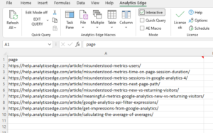
 When you use Analytics Edge in the Interactive mode, the data from the selected workbook is available for the wizard you open. For some wizards, like the new Google Search connector’s URL Inspection query, this allows you to process multiple URLs at once.
To select Interactive mode, simply check the box in the Analytics Edge ribbon (see the image above). Make sure to select the worksheet cell at the top left corner of the worksheet data you want to use (e.g. cell A1) — the add-in will automatically read the data from that point.
Then open the wizard for the function or query you want to run. For example, if you try a Google Search connector URL Inspection query, you will see the add-in loads the data from your worksheet and makes it available to the query (the green data showing behind the wizard).

In the query wizard, we can reference the data by entering a column name enclosed in square brackets (like an Excel range name: ‘[page]’). Most wizards will only accept a single value, in which case the top or first value will be used. In some wizards, though, like the URL Inspection query, they are designed to accept a list of values, and they will be fed all the values in the column.
Once the function or query is finished, the add-in will ask what you want to do with the results. You are offered the option to overwrite the original data, create a new worksheet with the results, or write the results to a specific location that you select.

Just before you do that, note that a sample of the results are showing in green behind the dialog, and if you want to repeat this sequence, you can check the box at the bottom of the dialog to save as an Analytics Edge macro.