Calculating a Weighted Average (Average of Averages)

A common reporting challenge in Excel is merging sets of data, such as combining monthly numbers for a quarterly or annual total. Adding up simple metrics is obvious, but what do you do with things like the average position or conversion rate? [Hint: you should not average or total anything that is already an average or ratio]

207,001 impressions with avg position of 35.7
+ 735,462 impressions with avg position of 55.1
= 942,463 impressions with avg position of ???

CTR is Click-Through-Rate; Position is Average Position

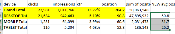
Our objective is to calculate the average position for each of the 3 device types in the fewest number of steps possible. A complication is that the 2 sets of data may be in different orders (desktop/mobile/tablet vs mobile/desktop/tablet), and some values may be missing from each data set (mobile/desktop).

The Lure of the Weighted Average

Rates and averages are calculated metrics, and they are all based on a sample or ‘population’ of data. In the example above, an average position of 35.7 (highlighted in yellow) is based on a specific group of 207,001 impressions. The actual math behind that average position involves adding up all the individual position values and dividing by the total number of impressions — that gives us an ‘average’:

avg position = (sum of positions) / (sum of impressions)

When combining calculated metrics like these, the size of each group is important — combining a small sample into a larger sample should not affect the overall average much (it should be closer to 55.1 than to 35.7 in the example above). What we want is a “weighted” average, where the size of the sample is taken into account when the numbers are combined. Searching for a typical formula for a weighted average yields something like this — you multiply each average by a weighting factor that is calculated from the proportion of the impressions they represent, then add them together:

weighted average = avg position1 * impressions1 / (impressions1 + impressions2) 
+ avg position2 * impressions2 / (impressions1 + impressions2)

Just describing it sounds complicated, and this formula is hard to implement, especially with large data sets. It would require looking up matching rows, then calculating the proportion or “weight”, then applying that to the avg position number, and finally adding them together. That is a lot of lookups and calculations, and it could be very slow.

Simplifying the Problem, and the Solution

In situations like this, we need to restate the problem in a way that is easier (faster) to solve. Going back to the simple formula for the average, we can assume that if the average position is the sum of positions divided by the number of impressions, then the average position for the combined data should be the sum of all of the positions, divided by the number of all of the impressions:

avg position = (sum of positions1 + sum of positions2) / (impressions1 + impressions2)

It sounds a lot simpler than the formula above, and if you are good at math formula substitutions, you can actually show this will result in exactly the same number. The difference is that it involves a number we don’t have in our data: the “sum of positions”. But that is easy enough to calculate; since the avg position is (sum of positions)/impressions, then we know:

sum of positions = avg position * impressions

Believe it or not, we now have a really simple way to combine our average with a few simple steps in a spreadsheet:

• append one data set to the other
• add a column calculating (avg position * impressions) called “sum of positions”
• combine duplicate rows, summing the numbers in matching rows (Sort and Subtotal in Excel)
• calculate a new avg position = (sum of positions)/(sum of impressions)

A Generic Approach

If you apply the same thinking to the click-through-rate (ctr) in a standard Google Search report, you will realize that you already have the clicks and impressions (they are default metrics) that are needed to calculate ctr (ctr = clicks/impressions). All you need to do is to append the data, combine the duplicate rows, then calculate the new ctr column from clicks/impressions.

The ‘extra’ step for the avg position in the first example exists because we did not start with one of the ‘base’ metrics behind the calculated metric — the (sum of positions). Going back to the step-by-step list, we can make it more generic:

• append one data set to the other
• if you need to combine calculated metrics (average, rate, percentage), then first break them down into their base metrics*
• combine duplicate rows, summing the numbers in every column
• recalculate the calculated metrics from the (summed) base metrics

* Note: if you can, include the base metrics in your query to eliminate the need for the second step. e.g. include Bounces and Sessions in your query instead of the Bounce Rate.

Base Metrics for Common Rates and Averages

Your first challenge is to figure out what the base metrics are for any rate or average metric you are using. You can then include those metrics in your query, or calculate them from the data you do have. Here are some of the common ones for Google Search and Google Analytics:

click-through rate = clicks / impressions
bounce rate = bounces / sessions
% new sessions = new users / sessions
avg session duration = session duration / sessions
goal conversion rate = goal completions / sessions
avg order value = revenue / sessions
ecommerce conversion rate = transactions / sessions

Summary

If you need to merge two or more sets of numbers and they include calculated metrics like averages, rates or percentages, make sure you combine them the right way. Don’t be put off by complicated formulas for weighted averages – the problem, and solution, is actually quite simple.

Start with (or calculate) the base metrics, combine (sum) the duplicate rows, and recalculate the calculated measures. Simple operations for accurate reporting.